Algorithms and Mathematical Background
Overview
electroMICA projects electrophysiological features (scalp or intracranial EEG) onto cortical and hippocampal surfaces using forward and inverse modeling techniques based on the Boundary Element Method (BEM).
Intracranial EEG (iEEG) Method

The main steps of the pipeline are: initial transformation of electrode positions to micapipe’s nativepro space, computation of sensitivity of iEEG channels to generators on cortical and hippocampal surfaces, and construction of cortical maps of input features. To compute the sensitivity of the SEEG channels to neuronal generators of electric activity at each node of the cortical surface, the electromagnetism equations governing the electric phenomena in the brain are solved with the Boundary Element Method (BEM). The head is modeled as a single layer given by the inner-skull surface, obtained from the brain mask. The generators of electric activity are modeled as a current density double layer on the cortical surface, linearly interpolated between the nodes.
von Ellenrieder et al. On the EEG/MEG forward problem solution for distributed cortical sources. Med Biol Eng Comput. 2009;47(10):1083-1091. doi:10.1007/s11517-009-0529-x
This model is different than usual models for distributed activity, avoiding mathematical singularities of multiple-dipole models with large numerical instabilities when the electrodes are close to the cortical surface. This more realistic and mathematical well-behaved model we adopt is unique to electro-MICA. The metallic contacts of the electrodes are modelled as a line with the true length of the contact, not a single point. The electric potential at the electrode is computed as the average potential along this line, with 5th order Gauss-Legendre quadrature.
The sensitivity of iEEG decreases very rapidly with the distance to the contacts. The sensitivity to generators far from the contacts is negligible compared to the measurement noise or masked by activity closer to the channel. Thus, two thresholds are applied for the constructions of the feature maps. A threshold common to all channels reflecting the effect of the noise (0.001 Vm/A), and a channel dependent relative threshold (0.05 of the maximum sensitivity of the channel). The sensitivity of each iEEG channel is computed based on the contact sensitivities. Finally, each node of the surfaces is assigned the value of the feature from the channel with highest sensitivity at that node (piecewise constant map) or a weighted average of the features with the weights given by the thresholded channel sensitivities. Large portions of the cortex are typically far from all iEEG contacts and will not be observable with iEEG. The maps show no value (NaN) for the surface vertices in these regions.

Scalp EEG Method
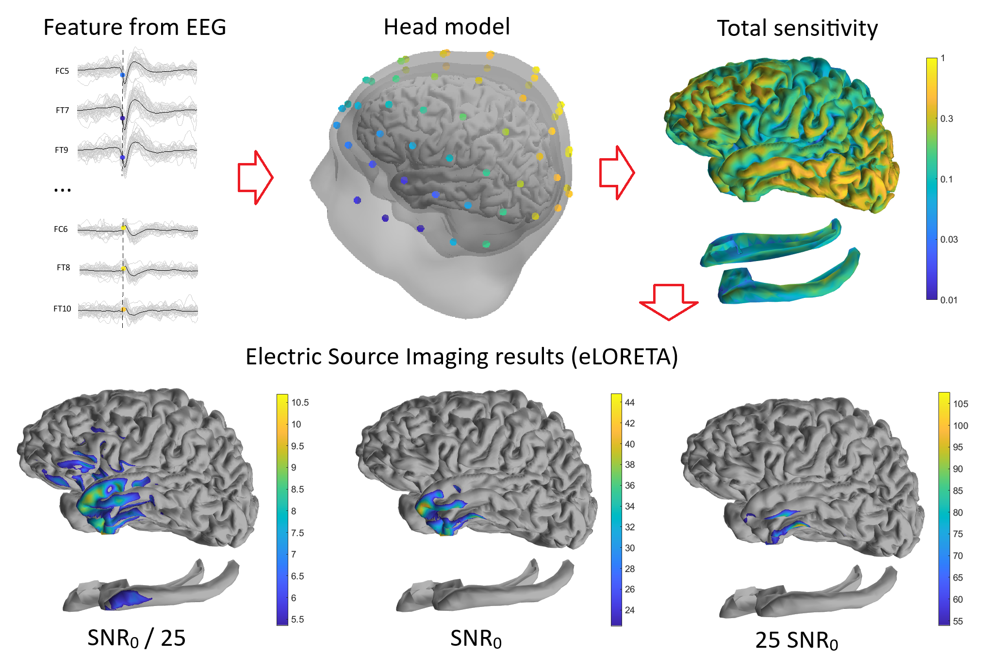
The head model is a three-layer model (brain, skull, skin) built from the T1-weighted volume in nativepro space from micapipe and its brain mask, through morphological processing. Anatomical landmarks in the pre-auricular points, nasion and inion, as well as the location of 10-10 scalp electrodes are approximated from the transformed positions in MNI152 space, projected onto the scalp surface of the subject. If non-standard electrode locations are used, the a registration based on anatomical landmarks is carried out. The generators of electric activity are modeled as distributed dipolar sheets on the cortical surfaces from micapipe, and optionally the hippocampal surfaces from HippUnfold. The forward problem is solved using BEM, and the source localization using eLORETA, with a smoothed covariance prior. Five different solutions are computed for each feature, corresponding to very-low, low, medium, high, and very-high signal-to-noise (SNR) values. The user can choose which corresponds to the data under analysis, from a single event almost completely masked by noise (very-low SNR, SNR0/25), to an extremely clear average of a large number of events in a good quality recording (very-high SNR, 25 SNR0).
Output Files
The pipeline generates:
Leadfield/Sensitivity matrices (.mat): Contains the leadfield matrix and other model information, output in /model.
Feature maps (.gii GIFTI): Vertex-wise projected features, output in /maps.
See Also
Usage — Practical usage examples
API Reference — Function reference